|
Ecopath with Ecosim (EwE)
EwE is used to characterise the trophic structure, ecosystem attributes, impact of fishing and other human uses and climate change in the region. It consists of a number of modules. Ecopath mass-balance model accounts for trophic interactions among organisms at multiple trophic levels by describing matter and energy flows. Ecosim and Ecospace uses the mass-balanced model generated by Ecopath to simulate dynamical changes due to human activities (including fishing), climate change and other time varying processes, as well as the effects of different management options, such as controls on fishing effort and spatial closures, on both fished species and the trophic interactions in the Kimberley marine ecosystem. More details about these modules can be found at http://www.ecopath.org/. An extensive list of references, showcasing the use of EwE on a number of ecological applications can be found here.
EwE model domain
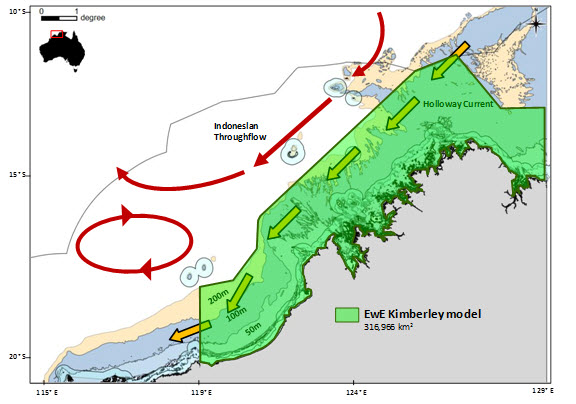
The geographical extent of EwE model domain can be seen in Figure 1 and the rationale for the choice of the domain boundaries is included in Table 1. At the core of these choices lies a distinction between two scales: i) the ‘jurisdictional’ scale at which Management Strategies apply and ii) the ‘geophysical/ecological’ scale at which Model Specification and Development Scenarios apply. To properly evaluate the impact of actions taken at the ‘jurisdictional’ scale, processes at the ‘geophysical/ecological’ scale need to be accounted for, since these will affect, and potentially invalidate, management interventions.
Figure 1 shows the EwE model domain. The rationale for this choice is more easily understood by analysing both the bathymetry and main ocean currents as in Figure 2 below.
 |
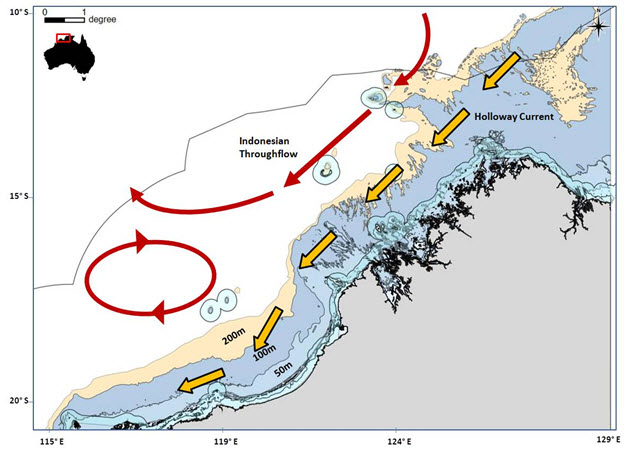 |
| Figure 1. The EwE Model Domain (left) and bathymetry and main ocean currents over the Kimberley region (right) |
| Model Boundary |
Rationale |
| North. It roughly follows the 200m depth contour |
It contains surface currents (Indonesian Throughflow; ITS) and seasonal currents (Holloway current) relevant for a better understanding of annual and inter-annual variability (ENSO/La Niña years) of primary production in the region.
The ITF and Holloway currents are related to the productivity of the Kimberley. For example, when the ITF is weak (El Niño events), the thermocline (60-100m depth on most areas) lifts bringing nutrient-rich waters into the photic zone and hence resulting in conditions favourable to increase primary productivity.
Seasonal variability of primary production due to wind and tidal actions occurring between 20-60m depth waters is considered.
Some internal waves (which can raise nutrient rich water via mixing) occur at 80-100m depths in the Kimberley region.
|
| West. 119°E, southern end of the Eighty-Mile Beach) |
This area contains more than 200 km2 of mudflats that are recognised as some of the most productive in the world, supporting an extraordinary rich benthic invertebrate community and one of the largest aggregations of shorebirds in the southern hemisphere.
This section of the model domain includes not only migratory birds, but also dugongs, turtles and sawfish. Humpback whales are sometimes seen in this area during their northern migration to calving grounds further along the Kimberley coast.
The Australian endemic snubfin dolphin (Orcaella heinsohni) inhabits this region. The extensive mangrove communities (north of Eighty-Mile Beach and Roebuck Bay) support important nursery areas for prawns, mudcrabs and fish.
Tourism and recreational fishing activities may increase in this area.
|
| East. Joseph Bonaparte Gulf, border with the Northern Territory. |
This region is characterised by its smooth bottom floor covered by soft, muddy sediments, which is significantly different from the rest of the Kimberley system.
Important influence of the ITF (warm and oligotrophic waters).
The Holloway Current has a presence here at the end of the Northwest Monsoon and also comprises surface waters at other times of the year.
Internal tides occur in this region, they are associated with upwellings.
Commercial prawn fishing occurs here.
Dugongs are known to be present and associated with seagrass communities in the inshore waters of the Gulf (i.e. waters <10m deep)) |
Structure of the Ecopath model
Defining EwE structure involves four main steps/components: i) a decision on what species should be included in the foodweb and ii) a characterisation of these species in terms of abundances, biological characteristics (growth, mortality, consumption, etc) and feeding relations, iii) a definition of the human-driven stressors on the system (fishing, tourism, etc.) and iv) the spatial relation among these components. As for any modelling choice, the level of details used to represent each component needs to reconcile the two competing needs of accounting for ecosystem complexity and simplifying our analysis to make it manageable. Finding a workable compromise requires both scientific knowledge and modelling experience.
Step (i) needs to be carried out first and is commonly done by selecting a minimum number of functional groups which satisfactory describe the behaviour of the overall foodweb. Here, a functional group is defined as a number of species of comparable ecological or feeding behaviour which can be treated as functionally similar. Which functional groups are selected is also determined by the purpose of the analysis as functional groups can at times include individual species of specific commercial or conservation interest.
Once the functional groups and their composition have been chosen, step (ii) needs to characterise these in terms of abundances, biological characteristics and diets. This is a time-consuming effort, since this information is rarely at hand and needs to be sought from disparate sources, often hard to locate. The output of this process, as discussed above, is a snapshot of what we know about the system and the data gaps highlight what we do not know about the system. A similar process is used to describe the human-driven stressors on the system in step (iii).
In addition, we provide a graphic summary of this information. It shows the network of interactions which EwE simulates. Each node represents either a functional group or a stressor. Each link represents the strength of the interaction between two nodes, be this predation, fishing or other stressor. Naturally, this network contains a lot of information, too much to be visualised at once. As a result, the network has a number of interactive features:
Moving the cursor over a node will display some basic information about that functional group, including its Pedigree, an assessment of how reliable this specific information is (see also Data Quality below)
Clicking on a node will highlight the network in the vicinity of the node. In particular this will display the links between the nodes and its neighbours.
it is also possible to zoom in and out and pan across the network to focus on specific components.
Functional group designation
Because of the enormous amount of differentiation in life-history, morphology and feeding guilds that appears within the Kimberley limestone reef fish families, delineating functional groups by fish family is impractical and may be unwise. The group structure in any particular EwE model is largely subjective and should be tailored to satisfy specific requirements of the investigation. Therefore, most of the functional groups developed for the preliminary Kimberley ecosystem model are based on the functional role that the fishes play in the ecosystem, with additional groups configured to allow the representation of important commercial, social and ecological interests. The Kimberley model contains 59 functional groups, including two non-living groups such as terrestrial inputs and organic detritus. A number of single species functional groups were defined for species of significance to commercial or recreational fishing fishers (e.g. Barramundi, Threadfin, Spanish mackerel). The model also represents marine mammals, sea birds, commercial and non-commercial invertebrates and plants. Table 1 presents the functional groups contained in the Kimberley model.
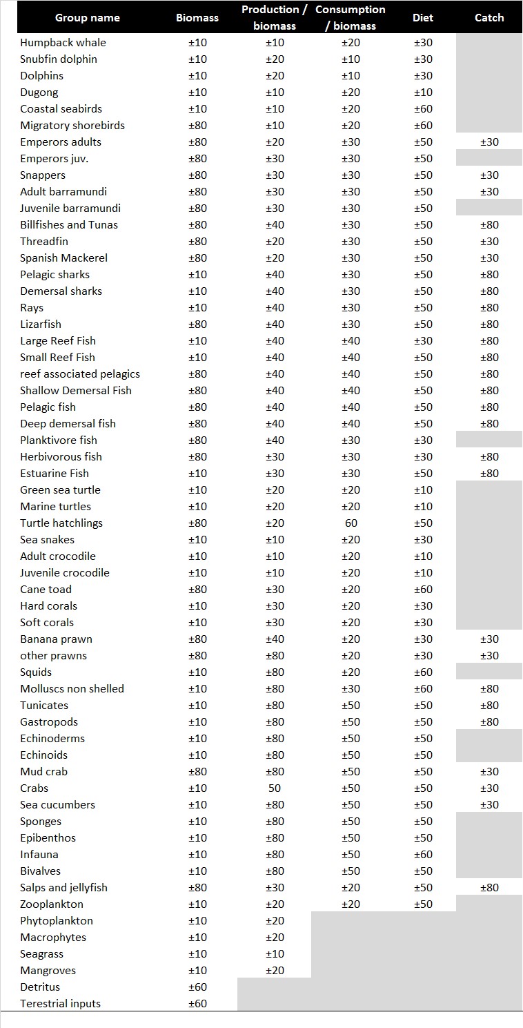
| Table 1. Input parameters for the Ecopath model: Biomass (B - t·km-2), production (P/B - year-1), consumption (Q/B - year-1), diet and catch. Colour codes (see legend) refer to data origin. Here it is assumed that, on average, local data (red) is more reliable than data obtained from sources outside the region, which include information from the literature, from empirical relationships or from other Ecopath models. Click here or on the image for a higher resolution version. |
| Description |
Group name |
Trophic level |
Habitat area |
Biomass in habitat |
Biomass |
P/B |
Q/B |
Ecotrophic efficiency |
|---|
| Marine mammals | Humpback whale | 2.8 | 0.6 | 4.5 | 2.7 | 0.017 | 2.7 | 0.11 |
| Snubfin dolphin | 3.8 | 1 | 0.115 | 0.115 | 0.04 | 70 | 0.66 |
| Dolphins | 3.7 | 1 | 0.1503 | 0.1503 | 0.04 | 70 | 0.75 |
| Dugong | 2.0 | 0.2 | 0.02 | 0.004 | 0.08 | 11 | 0.76 |
| Birds |
Coastal seabirds | 2.7 | 1 | 0.081 | 0.081 | 5.6 | 65 | 0.99 |
| Migratory shorebirds | 2.4 | 0.6 | 0.0104 | 0.00624 | 5.4 | 80 | 0.89 |
| Empeors adults | 2.7 | 1 | 0.017 | 0.017 | 0.44 | 4.5 | 0.95 |
| Empeors juvenile | 2.5 | 1 | 0.077 | 0.077 | 0.91 | 7.2 | 0.95 |
| Snappers | 2.9 | 1 | 0.130 | 0.130 | 0.32 | 5.33 | 0.95 |
| Adult Barramundi | 3.4 | 1 | 0.111 | 0.111 | 1.46 | 5.7 | 0.95 |
| Juvenile Barramundi | 2.2 | 1 | 0.442 | 0.442 | 1.85 | 7.81 | 0.95 |
| High commercial species |
Billfishes and Tunas | 3.6 | 1 | 0.011 | 0.011 | 0.41 | 7.14 | 0.95 |
| Threadfin | 2.9 | 1 | 0.013 | 0.013 | 1.12 | 4.1 | 0.95 |
| Spanish Mackerel | 3.5 | 1 | 0.025 | 0.025 | 0.52 | 6.8 | 0.95 |
| Pelagic sharks | 3.5 | 1 | 0.0076 | 0.0076 | 0.33 | 5.2 | 0.09 |
| Demersal sharks | 2.9 | 1 | 0.0767 | 0.0767 | 0.33 | 3.8 | 0.52 |
| Predator fish |
Rays | 3.5 | 1 | 0.00110 | 0.00110 | 0.19 | 2.44 | 0.75 |
| Lizarfish | 2.9 | 1 | 0.12 | 0.12 | 0.74 | 7.1 | 0.95 |
| Large Reef Associated | 2.2 | 0.5 | 6.71 | 3.355 | 0.54 | 23.5 | 0.98 |
| Small Reef Associated | 2.7 | 1 | 7.110 | 7.110 | 0.71 | 29.05 | 0.95 |
| Other fish |
Reef Associated Pelagics | 2.3 | 0.4 | 4.974 | 1.990 | 3.1 | 28.06 | 0.95 |
| Shallow demersal fish | 3.1 | 0.5 | 6.862 | 3.431 | 0.78 | 11.63 | 0.95 |
| Pelagic fish | 2.4 | 0.7 | 1.857 | 1.300 | 0.4 | 7 | 0.95 |
| Deep Demersal fish | 2.3 | 0.4 | 0.924 | 0.370 | 0.75 | 11.5 | 0.95 |
| Planktivore fish | 2.0 | 0.8 | 1.590 | 1.272 | 2.25 | 10.21 | 0.95 |
| Herbivorous fish | 2.1 | 0.3 | 64.78 | 19.43 | 2.15 | 9.7 | 0.95 |
| Estuarine fish | 2.0 | 0.05 | 176.600 | 8.830 | 2.46 | 12.8 | 0.87 |
| Green sea turtle | 2.5 | 1 | 0.00391 | 0.00391 | 0.06 | 11 | 0.41 |
| Marine turtles | 2.5 | 1 | 0.064 | 0.064 | 0.07 | 11 | 0.70 |
| Turtle hatchlings | 3.4 | 0.3 | 1.423 | 0.427 | 12.22 | 17.77 | 0.95 |
| Reptiles |
Sea snakes | 3.4 | 1 | 0.001 | 0.001 | 0.46 | 6.3 | 0.23 |
| Adult crocodile | 3.0 | 0.3 | 1.792 | 0.5376 | 0.15 | 5.7 | 0.03 |
| Juveniles crocodiles | 3.1 | 0.6 | 0.183 | 0.110 | 0.48 | 13.3 | 0.77 |
| Invasive species | Cane toad | 2.6 | 0.2 | 3.66 | 0.73 | 2 | 20 | 0.10 |
| Corals |
Hard coral | 2.6 | 0.25 | 15.89 | 3.9725 | 0.12 | 12 | 0.62 |
| Soft coral | 2.1 | 0.25 | 24.68 | 6.17 | 0.9 | 0.9 | 0.81 |
| Other invertebrates | Banana prawns | 2.1 | 1 | 0.010 | 0.010 | 4.4 | 18.2 | 0.95 |
| Other prawns | 2.1 | 1 | 0.12 | 0.12 | 3.2 | 18.2 | 0.95 |
| Squids | 2.9 | 1 | 0.34 | 0.34 | 4.05 | 17.9 | 0.95 |
| Molluscs non shelled | 2.7 | 1 | 0.126 | 0.126 | 3.5 | 12.5 | 0.95 |
| Tunicates | 2.3 | 0.35 | 32.82 | 11.487 | 0.24 | 32 | 0.95 |
| Gastropods | 2.4 | 1 | 0.961 | 0.961 | 3.9 | 10 | 0.95 |
| Echinoderms | 2.4 | 1 | 7.78 | 7.78 | 1.8 | 6 | 0.95 |
| Echinoids | 2.0 | 0.2 | 26.1 | 5.22 | 4.6 | 8.5 | 0.95 |
| Mud crab | 2.1 | 1 | 0.111 | 0.111 | 2.7 | 9.5 | 0.95 |
| Crabs | 2.1 | 1 | 0.461 | 0.461 | 4.1 | 19 | 0.95 |
| Sea cucumbers | 2.2 | 1 | 0.96 | 0.96 | 0.7 | 2.07 | 0.95 |
| Sponges | 2.4 | 1 | 12.19 | 12.19 | 0.24 | 30.21 | 0.95 |
| Epibenthos | 2.1 | 1 | 7.89 | 7.89 | 2.9 | 10 | 0.95 |
| Infauna | 2.0 | 1 | 0.721 | 0.721 | 3.95 | 14 | 0.95 |
| Bivalves | 2.2 | 1 | 0.008 | 0.008 | 3.9 | 10 | 0.95 |
| Nekton |
Salps & Jellyfish | 2.4 | 1 | 1.12 | 1.12 | 20 | 40 | 0.95 |
| Zooplankton | 2.0 | 1 | 36.54 | 36.54 | 55 | 70 | 0.91 |
| Primary producers | Phytoplankton | 1.0 | 1 | 41.87 | 41.87 | 90 | | 0.99 |
| Macrophytes | 1.0 | 1 | 2.51 | 2.51 | 24 | | 0.96 |
| Seagrass | 1.0 | 0.2 | 75.87 | 15.174 | 9.8 | | 0.96 |
| Mangroves | 1.0 | 0.3 | 0.880 | 0.264 | 0.02 | | 0.76 |
| Non living | Organic detritus | 1.0 | 1 | 20 | 20 | | | 0.96 |
| Terrestrail inputs | 1.0 | 0.1 | 10 | 1 | | | 0.40 |
|
Input data and information sources
This section describes the general methodology used to assign functional groups their basic parameters required by the EwE model. The data needs of EwE can be summarized as follows. Four data points are required for each functional group: biomass (in t·km-2), the ratio of production over biomass (P/B; in yr-1), the ratio of consumption over biomass (Q/B; in yr-1), and ecotrophic efficiency (EE; unitless). EwE also provides an input field representing the ratio of production over consumption (P/Q; unitless), which users may alternatively use to infer either P/B or Q/B based on the other. Each functional group requires 3 out of 4 of these input parameters and the remaining parameter is estimated using the mass-balance relationship in equations 1 and 2. A biomass accumulation rate may be entered optionally; the default setting assumes a zero-rate instantaneous biomass change. These EwE data points are referred to collectively in this report as the basic parameters. For further details of EwE data needs and parameter definitions see Christensen et al., (2004). Most often, Q/B was set using the empirical formulae of Christensen and Pauly (1992); a few species were set using Palomares and Pauly (1998) using tail aspect ratio as modified by Christensen et al. (2004). P/B was determined based on the sum of the natural mortality rate (M), estimated using the empirical formula of Pauly (1980), and some fishing mortality rate (F) which is an assumed fraction of M. As a guideline, heavily exploited species were assumed to have an F approximately equal to M, while moderately exploited species were assumed (for most of the cases) to have an F equal to M/2 or less.
We present here how the functional group parameterization was obtained (reporting where literature values and other special data sources were used to set the basic parameters). The sources of data for basic input parameters for each functional group and species in the model are summarized in Table 2. Parameter estimates came from the study region wherever possible, mainly by other studies conducted during 2013-2016 by WAMSI-2 research projects (Table 2).
| Table 2. Information sources of the main input parameters of the Ecopath with Ecosim model for the marine region of the Kimberley, biomass (B), production:biomass ratio (P/B), consumption:biomass ration (Q/B) and diet. Click here or on the image for a higher resolution version. |
| Trophic Group | infoB | infoP/B | infoQ/B | infoDiet |
|---|
| Humpback whale | Blake et al. 2011 | Holyoake et al., 2012 | Holyoake et al., 2012 | Holyoake et al., 2012 |
| Snubfin dolphin | Brown et al., 2016 | Beasley et el., 2005 | Brown et al., 2013 | Beasley et el., 2005 |
| Dolphins | Brown et al., 2013 | Mann et al., 2000 | Krützen, 2014 | Krützen, 2014 |
| Dugong | Bayliss et al., 2016 | Marsh 2000 | Andre and Lawler, 2003 | Andre and Lawler, 2003 |
| Coastal seabirds | Watson et al., 2009 | Watson et al., 2009 | Jaquement et al., 2008 | Jaquement et al., 2008 |
| Migratory shorebirds | Watson et al., 2009 | Watson et al., 2010 | Jaquement et al., 2008 | Jaquement et al., 2008 |
| Empeors adults | Ecopath | Newman and Dunk, 2002 | Westera 2003 | Westera 2003 |
| Empeors juvenile | Ecopath | Westera 2003 | Westera 2003 | www.fishbase.org |
| Snappers | Ecopath | O'Neill et al., 2011 | O'Neill et al., 2012 | O'Neill et al., 2013 |
| Adult Barramundi | Ecopath | Griffin 1994 | Griffin 1994 | DoFWA 2014 |
| Juvenile Barramundi | Ecopath | Barlow et al, 1995 | Griffin 1994 | www.fishbase.org |
| Billfishes and Tunas | Ecopath | Hampton 2011 | Griffiths et al., 2009 | Griffiths et al., 2009 |
| Threadfin | Ecopath | Pember et al., 2005 | Pember et al., 2005 | www.fishbase.org |
| Spanish Mackerel | Ecopath | McPherson 1993 | McPherson 1993 | McPherson 1993 |
| Pelagic sharks | RPS 2011 | Pauly, 1980 | Stevens and McLoughlin 1991 | Stevens and McLoughlin 1991 |
| Demersal sharks | RPS 2011 | Pauly, 1980 | Stevens and McLoughlin 1991 | Stevens and McLoughlin 1991 |
| Rays | RPS 2011 | Pauly, 1980 | Pauly, 1980 | www.fishbase.org |
| Lizarfish | Ecopath | Pauly, 1980 | Pauly, 1980 | Ibrahim et al., 2003 |
| Large Reef Associated | Newman et al. 2004 | Connel, 1996 | Pauly, 1980 | www.fishbase.org |
| Small Reef Associated | Newman et al. 2004 | Connel, 1996 | Pauly, 1980 | www.fishbase.org |
| Reef Associated Pelagics | Ecopath | Connel, 1996 | Pauly, 1980 | Lek et al., 2011 |
| Shallow demersal fish | Ecopath | Pauly, 1980 | Pauly, 1980 | www.fishbase.org |
| Pelagic fish | Ecopath | Hewitt and Hoening, 2005 | Pauly, 1980 | www.fishbase.org |
| Deep Demersal fish | Ecopath | Pauly, 1980 | Pauly, 1980 | www.fishbase.org |
| Planktivore fish | Ecopath | Pauly, 1980 | Pauly, 1980 | www.fishbase.org |
| Herbivorous fish | Ecopath | Hart and Russ, 1996 | Hart and Russ, 1996 | www.fishbase.org |
| Estuarine fish | Newman et al. 2004 | Lorenzen, 1996 | Lorenzen, 1996 | www.fishbase.org |
| Green sea turtle | Bayliss et al., 2016 | Poiner and Harris, 1996 | RPS 2010 | Burkholder et al., 2013 |
| Marine turtles | RPS 2011 | Poiner and Harris, 1996 | RPS 2010 | Burkholder et al., 2013 |
| Turtle hatchlings | Ecopath | Gyuris, 1994 | Fulton et al. 2011 | Boyle and Limpus 2008 |
| Sea snakes | RPS 2011 | Milton, 2001 | Voris and Jayne, 1979 | Wirsing and Heithaus, 2009 |
| Adult crocodile | Halford 2016 | Halford 2016 | Webb, 1978 | Whiting and Whiting, 2011 |
| Juveniles crocodiles | Halford 2016 | Halford 2016 | Webb, 1978 | Whiting and Whiting, 2012 |
| Cane toad | Ecopath | Pine and Kwak 2007 | Pine and Kwak 2007 | Dam et al., 2002 |
| Hard coral | Keesing et al., 2011 | McClanahan et al., 2004 | McClanahan et al., 2004 | Ribes and Coma, 1998 |
| Soft coral | Keesing et al., 2011 | Baird and Marshall, 2002 | Baird and Marshall, 2002 | Fabricius et al., 2007 |
| Banana prawns | Ecopath | Gourguet et al., 2016 | Gourguet et al., 2016 | Gourguet et al., 2016 |
| Other prawns | Ecopath | Ecopath | Kienle et al., 2016. | Kienle et al., 2016. |
| Squids | Keesing et al., 2011 | Ecopath | Chembian and Mathew 2016 | Chembian and Mathew 2016 |
| Molluscs non shelled | WAMSI 2015 | Ecopath | Pauly et al 1993 | Loneragan et al. 2011 |
| Tunicates | WAMSI 2015 | Ecopath | Pauly et al 1993 | Sutherland et al., 2010 |
| Gastropods | WAMSI 2015 | Ecopath | Pauly et al 1993 | Compton et al., 2008 |
| Echinoderms | WAMSI 2015 | Ecopath | Pauly et al 1993 | Le Bourg e t al., 2016 |
| Echinoids | WAMSI 2015 | Ecopath | Andrew 1993 | Andrew 1993 |
| Mud crab | Ecopath | Pauly et al., 1993 | Pauly et al 1993 | Bustamante et al. 2010 |
| Crabs | WAMSI 2015 | Ecopath | Pauly et al 1993 | Laptikhovsky et al 2016 |
| Sea cucumbers | WAMSI 2015 | Ecopath | Pauly et al 1993 | Hamel et al, 2001 |
| Sponges | WAMSI 2015 | Ecopath | Pauly et al 1993 | Bustamante et al. 2010 |
| Epibenthos | Keesing et al., 2011 | Ecopath | Pauly et al 1993 | Lemloh et al, 2009 |
| Infauna | Keesing et al., 2011 | Ecopath | Pauly et al 1993 | Long et al., 1994 |
| Bivalves | Fry et al., 2008. | Ecopath | Pauly et al 1993 | Way et al., 1990. |
| Salps Jellyfish | Ecopath | Pitt et al., 2014 | Pitt et al., 2013 | Graham and Kroutil, 1989 |
| Zooplankton | Hollyday et el. 2011 | Kimmerer and McKinnon, 1987 | Kimmerer and McKinnon, 1987 | Hiltunen et al., 2015 |
| Phytoplankton | Blondeau-Patisser et al. 2011 | Chatterjee and Pal, 2016 | | |
| Macrophytes | Fry et al., 2008. | Short et al., 2015 | | |
| Seagrass | Kendrick et al., 2016 | Kendrick et al., 2016 | | |
| Mangroves | PTTEP Australasia, 2013 | Ward et al., 2016 | | |
| Organic detritus | Ecopath | | | |
| Terrestrail inputs | Ecopath | | | |
|
Diet composition
The diet composition matrix was assembled as percentage weight or volume of the annual fraction that each prey contributes to the overall diet of the predator (according to the methodology recommend by Christensen et al., 2004). Several local reports were employed to assemble this matrix of feeding interactions, but when data from the Kimberley was not specifically available, values were taken from the same species from the adjacent areas (North West Shelf, Ningaloo, Gulf of Carpentaria). The diet composition matrix of the mass-balanced model underlays the network relation shown here as described above.
Fisheries
Gear types
The fishing gear types included the Kimberley model were selected based on the operating fleets reported in the region by Department of Fisheries, WA. The gear structure proposed for the model included seven gear types for both commercial and recreational fisheries. A total of five gear types represent the commercial fisheries of the region with the following gears: Kimberley Prawn Managed Fishery, Kimberley Gillnet and Barramundi Managed Fishery, Broome Prawn Managed Fishery, Mackerel Fishery, and Northern Demersal Scalefish. In the case of recreational fishing, the following two gears are included in the model: boat and beach anglers, and Beche-de-mer.
Commercial Catch
Most of the commercial fisheries catch data used in the model were estimated from the fisheries statistics reported by the Department of Fisheries, Western Australia. The fisheries data included the total catch (tonnes), gear types and species fished within each of the relevant districts in which the Department of Fisheries manages and reports fisheries statistics in Western Australia. According to this organization, the region of the Kimberley is included in the North Coast Bioregion. The commercial fisheries in this region are focused on the tropical snappers in offshore waters and barramundi, threadfin salmon, and shark in more coastal areas. Most of the Western Australia states smaller prawn trawl fisheries are also based in this region. Table 3 presents the commercial catch included in the model from the main five fleets operating in the Kimberley from 2010 to 2014.
| Table 3. Mean commercial and recreational catch (t ·km-2) from 2012 to 2014 estimated for the EwE Kimberley model domain based on data provided by Department of Fisheries WA |
| Group/fleet | Kimberley Prawn Managed Fishery | Kimberley Gillnet and Barramundi Managed Fishery | Broome prawn Managed Fishery | Mackerel Fishery | Northern Demersal Scalefish | Recreational fishing | Beche-de-mer |
|---|
| Humpback whale | 0 | 0 | 0 | 0 | 0 | 0 | 0 |
| Snubfin dolphin | 0 | 0 | 0 | 0 | 0 | 0 | 0 |
| Dolphins | 0 | 0 | 0 | 0 | 0 | 0 | 0 |
| Dugong | 0 | 0 | 0 | 0 | 0 | 0 | 0 |
| Coastal seabirds | 0 | 0 | 0 | 0 | 0 | 0 | 0 |
| Migratory shorebirds | 0 | 0 | 0 | 0 | 0 | 0 | 0 |
| Empeors adults | 0.000444591 | 0 | 0 | 4.45E-05 | 0.04103576 | 0.0965652 | 0 |
| Empeors juvenile | 8.13E-05 | 0 | 0 | 0 | 0 | 0 | 0 |
| Snappers | 0 | 0 | 0 | 0 | 0 | 0.03665321 | 0 |
| Adult Barramundi | 0 | 0.05866691 | 0 | 0 | 0 | 0.09288928 | 0 |
| Juvenile Barramundi | 0 | 0 | 0 | 0 | 0 | 0.000388206 | 0 |
| Billfishes and Tunas | 0 | 0 | 0 | 0.01257748 | 0 | 0.009215183 | 0 |
| Threadfin | 0 | 0.00806714 | 0 | 0 | 0 | 0.1864766 | 0 |
| Spanish Mackerel | 0 | 0 | 0 | 0 | 0 | 0.04401238 | 0 |
| Pelagic sharks | 0 | 0.01690217 | 0 | 0.001154806 | 0 | 0.000810464 | 0 |
| Demersal sharks | 0 | 0 | 0 | 0 | 0.05450065 | 0.000249129 | 0 |
| Rays | 0.000956749 | 0 | 0 | 0 | 0 | 0 | 0 |
| Lizarfish | 0 | 0 | 0 | 0 | 0 | 6.66E-05 | 0 |
| Large Reef Associated | 0 | 0 | 0 | 0 | 0 | 0.000522052 | 0 |
| Small Reef Associated | 0 | 0 | 0 | 0 | 0 | 0.000858682 | 0 |
| Reef Associated Pelagics | 0 | 0 | 0 | 0 | 0 | 0.002124104 | 0 |
| Shallow demersal fish | 0 | 7.78E-06 | 0 | 0 | 2.29E-06 | 7.11E-05 | 0 |
| Pelagic fish | 0 | 7.32E-06 | 0 | 7.32E-07 | 7.32E-06 | 0.002999601 | 0 |
| Deep Demersal fish | 0 | 0 | 0 | 2.55E-06 | 0.000254722 | 0 | 0 |
| Planktivore fish | 0 | 0 | 0 | 0 | 0 | 0 | 0 |
| Herbivorous fish | 0 | 0 | 0 | 0 | 0 | 4.82E-05 | 0 |
| Estuarine fish | 0 | 0 | 0 | 0 | 0 | 1.51E-05 | 0 |
| Green sea turtle | 0 | 0 | 0 | 0 | 0 | 0 | 0 |
| Marine turtles | 0 | 0 | 0 | 0 | 0 | 0 | 0 |
| Turtle hatchlings | 0 | 0 | 0 | 0 | 0 | 0 | 0 |
| Sea snakes | 0 | 0 | 0 | 0 | 0 | 0 | 0 |
| Adult crocodile | 0 | 0 | 0 | 0 | 0 | 0 | 0 |
| Juveniles crocodiles | 0 | 0 | 0 | 0 | 0 | 0 | 0 |
| Cane toad | 0 | 0 | 0 | 0 | 0 | 0 | 0 |
| Hard coral | 0 | 0 | 0 | 0 | 0 | 0 | 0 |
| Soft coral | 0 | 0 | 0 | 0 | 0 | 0 | 0 |
| Banana prawns | 0.002601935 | 0 | 0 | 0 | 0 | 0 | 0 |
| Other prawns | 0.000467712 | 0 | 0.0183395 | 0 | 0 | 0 | 0 |
| Squids | 0 | 0 | 0 | 0 | 0 | 0 | 0 |
| Molluscs non shelled | 7.78E-06 | 0 | 0 | 0 | 0 | 0 | 0 |
| Tunicates | 0 | 0 | 0 | 0 | 0 | 0 | 0 |
| Gastropods | 0 | 0 | 0 | 0 | 0 | 0 | 0 |
| Echinoderms | 0 | 0 | 0 | 0 | 0 | 0 | 0 |
| Echinoids | 0 | 0 | 0 | 0 | 0 | 0 | 0 |
| Mud crab | 0 | 0 | 0 | 0 | 0 | 7.14E-05 | 0 |
| Crabs | 3.34E-06 | 0 | 0 | 0 | 0 | 0 | 0 |
| Sea cucumbers | 0 | 0 | 0 | 0 | 0 | 0 | 0.000117327 |
| Sponges | 0 | 0 | 0 | 0 | 0 | 0 | 0 |
| Epibenthos | 0 | 0 | 0 | 0 | 0 | 0 | 0 |
| Infauna | 0 | 0 | 0 | 0 | 0 | 0 | 0 |
| Bivalves | 0 | 0 | 0 | 0 | 0 | 0 | 0 |
| Salps Jellyfish | 6.42E-06 | 0 | 0 | 0 | 0 | 0 | 0 |
| Zooplankton | 0 | 0 | 0 | 0 | 0 | 0 | 0 |
| Phytoplankton | 0 | 0 | 0 | 0 | 0 | 0 | 0 |
| Macrophytes | 0 | 0 | 0 | 0 | 0 | 0 | 0 |
| Seagrass | 0 | 0 | 0 | 0 | 0 | 0 | 0 |
| Mangroves | 0 | 0 | 0 | 0 | 0 | 0 | 0 |
| Organic detritus | 0 | 0 | 0 | 0 | 0 | 0 | 0 |
| Terrestrail inputs | 0 | 0 | 0 | 0 | 0 | 0 | 0 |
|
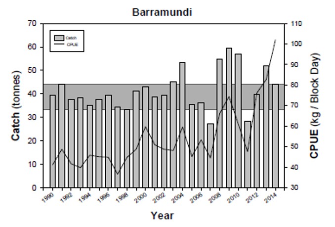
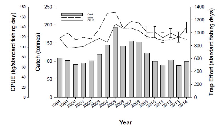
Kimberley Gillnet and Barramundi Managed Fishery (KGBF)
| The Kimberley Gillnet and Barramundi Managed Fishery extends from the WA/NT border to the top of Eighty Mile Beach, south of Broome (Latitude 19°S). It encompasses the taking of fish by means of gillnet and the taking of barramundi by any means. The species taken are predominantly barramundi (Lates calcarifer) and threadfin salmon (Eleuthronema tetradactylum). The main areas of the fishery are the river systems of the northern Kimberley, the Fitzroy River, Roebuck Bay and Eighty Mile Beach. This figure 2.4 presents the annual catch and catch per unit of effort (CPUE, kg block day-1) for barramundi caught for the KGBF over the period 1990 to 2014 (Data from Department of Fisheries, WA). |
 |
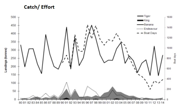
Kimberley Prawn Managed Fishery
| The Kimberley Prawn Managed Fishery operates off the north of the State adjacent to the Commonwealth-Managed Northern Prawn Fishery. The boundaries of tis fishery are all Western Australian waters of the Indian Ocean lying east of 123°45 east longitude and west of 128°58 east longitude (Department of Fisheries, 2014). A significant number of vessels hold authorisations to operate in both fisheries, and opening and closing dates are aligned to prevent large shifts of fishing effort into the Kimberley fishery. This figure presents the annual landings and number of boat days for the Kimberley Prawn Managed Fishery from 1980 to 2014 (Data from Department of Fisheries, WA). |
 |
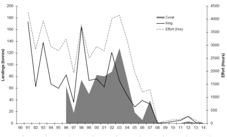
Broome Prawn Managed Fishery
| The Broome Prawn Managed Fishery is a small fishery which operates in July-August in a designed trawl zone off Broome and generally coincides with the seasonal closures of the northern and Kimberley prawn fisheries. The dominant species caught are western king prawns (Penaeus latisulcatus) and coral prawns (a combined category for small penaeid species). This figure presents the annual landings and fishing effort for the Broome Prawn Managed Fishery from 1991 to 2014 (Data from Department of Fisheries, WA). |
 |
Northern Demersal Scalefish Managed Fishery
| The Northern Demersal Scalefish Managed Fishery (NDSF) operates off the north-west coast of Australia in the waters east of 120°E longitude. These waters extend out to the edge of the Australian Fishing Zone (200 nautical mile). Commercial catches are dominated by tropical snappers, emperors, cods and gropers by the use of fish traps, and to lesser extend line fishing methods such as handline and/or dropline. This figure presents the catch, effort and catch per unit of effort of red emperor in the NDSF by trap from 1998 to 2014 (Data from Department of Fisheries, WA). |
 |
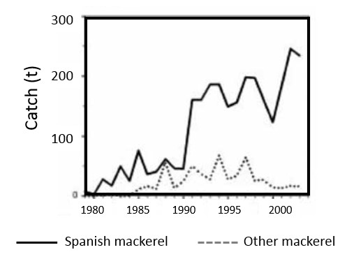
Spanish Mackerel Fishery
| Fishing for Spanish mackerel (Scomberomorus commerson), under the general wetline access available to all Western Australian licensed commercial fishing boats. Spanish mackerel are usually capture at or near the surface in coastal areas around reefs, headlands and shoals (Department of Fisheries, 2014). The use of dories (5-6.5m dinghies) is restricted to the Kimberley sector, which extends east of longitude 121°E to the NT border. Dories troll two or three lines and work to a mother boat that is about 20m in length. Fishing gear used in this sector is relatively heavy (8-10mm rope with 200+kg mono line and wire trace), crews number between one and five, and fishing trips generally last between one and three weeks. Thsi figure presents the annual catches of Spanish mackerel and other mackerel in each sector of this fishery from 1979 to 2003. Other mackerel includes grey, school, spotted and shark mackerel (Data from Department of Fisheries, WA). |
 |
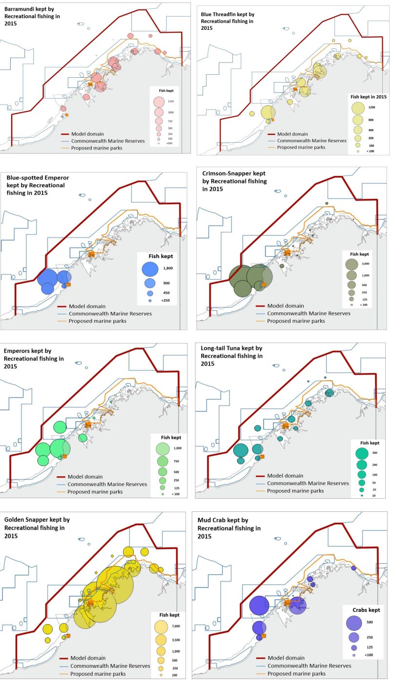
Recreational Catch
| Recreational fishing for finfish in the region (e.g. Barramundi, Threadfin, Snappers, Emperors) is also a significant activity. Only one gear of recreational fishing is included in the model: Recreational fishing which includes beach anglers, boat anglers, netting, diving and spear fishing. The recreational catch for the main finfish and invertebrate species targeted in the Kimberley were obtained from the data provided by the Department of Fisheries WA. The figure below presents the number of fish and crabs kept by recreational fishers in 2015. The recreational catch was estimated as 3,780 tonnes (0.044 t/km2). Table 4 presents the recreational catch estimated included in the model. |
 |
Model and data quality
| The pedigree routine in EwE serves as a sensitivity analysis for documenting the effect of inputs on estimated parameters and their quality. It calculates the 'pedigree index' (P) which measures the amount of local data used (i.e., minor uncertainty in the inputs) among the five basic categories of models: Biomass (B), Production to biomass (P/B), the ratio of consumption to biomass (Q/B), and diets and catches for each of the functional groups. The range of P is from 0 for data not rooted locally to 1.0 for data that are fully rooted in local data (Christensen et al., 2004).
The pedigree index provides confidence intervals for the input data of the model assuming that parameters originating from local data are of higher quality than those originating from other systems or guesstimates. The confidence intervals associated to each of these parameters were defined by the default values based on actual estimates of confidence intervals in various studies as reported by Christensen et al., 2000, as shown on the right hand side. Specifying the pedigree of data to generate Ecopath input is useful because, among other reasons, it provides a basis for the computation of an overall index of the model quality; a model of high quality when it is constructed mainly using precise estimates of various parameters, based on data from the system to be represented by the model. |
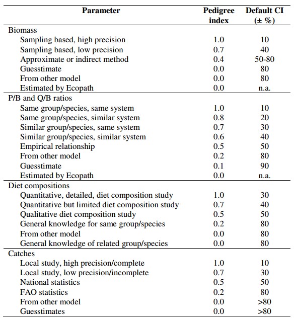 |
Table 4 presents the confidence intervals of the input data used in Kimberley model based on the pedigree index of EwE.
| Table 4. Confidence intervals (±CI%) for each functional group based on the origin of the five major categories of input parameters of the model: biomass, production/biomas, consumption/biomass, diet compostion and catches. |
 |
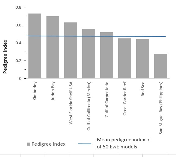
The figure below presents a comparison of the pedigree index (P) and its measure of fit (t*) of the Kimberley model with those reported in other Ecopath models. These indices indicate that the Kimberley model has been cosntructed with a very reliable data ganarated from local samplings. The Kimberley model has an overall pedigree of 0.73; in comparison, the analysis of 50 other models with an average of 27 groups resulted in a mean pedigree of 0.44 (Table 2.7; Morissette, 2007). This indicates that the Kimberley model is above about the quality data in terms of its uncertainty. This contrastd with the general perception that the Kimberley is a system underestudied.
 |
 |
| Comparison of the pedigree index of the Kimberley model with those reported in other EwE models (grey bars). The blue line represents the mean pedigree index of 50 Ewe models reported by Morisstte (2007). This index indicates that the Kimberley model has been constructed with a very reliable data generated from local samplings. |
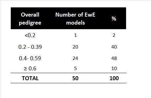
Number of EwE models for different levels of quality (pedigree) from Morissette 2007. |
Pre-balance (PREBAL) diagnostics
Once we collected the input data of the model, we run a set of PREBAL diagnostics including the slopes of biomass ratios, vital rates, total production and consumption based on trophic levels. These diagnostics are based on biological and fisheries principles and are recommended before a model is balanced (Heymans et al., 2016). The model has been evaluated for the quality of the input data through the following PREBAL diagnostics:
Biomass per trophic level
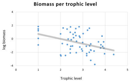
| The PREBAL criteria include the distribution of biomass per trophic level. It is expected that the slope of the biomass (on a log scale) decline by 5-10% across all the taxa arrayed by trophic level (Link, 2010). The PREBAL Kimberley model displayed a declining slope of the biomass (see figure to the right). Values above and below the slope-line were checked for data integrity before initiate the mass-balance of the model. This plot diagnostics shows that biomass estimates of shallow demersal fish, pelagic fish, planktivore fish, lizarfish, reef associated pelagic fish and herbivorous fish might potentially be over-estimated in the model, while that of threadfin, pelagic sharks, green turtle, turtle hatchings might be underestimated. The biomass estimates of these groups were checked before the mass-balancing, especially for the top predators. |
 |
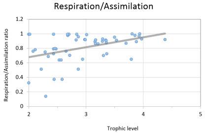
Respiration/Assimilation Biomass (RA/AS) <1.0
| The proportion of biomass lost through respiration cannot be higher than the biomass of food assimilated. As a rule of thumb. R-selected species (short life spans, lower trophic levels) are more likely to invest a large energy intake into growth and reproduction resulting in an RA/AS ratio below 1.0. In contrast, K-selected species (long-life spans, higher trophic levels) are expected to invest a relatively small proportion of energy intake in somatic and gonadal tissue production, are expected to have ratios close to 1.0. In the PREBAL Kimberley model the higher values of RA/AS ratios were displayed by the higher trophic groups, and as expected, values of RA/AS lower than 1.0 were showed by the groups within trophic level of two and three. |
 |
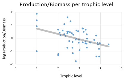
Annual Production/Biomass (P/B)
| In the model, the instantaneous mortality equals total production over mean biomass (Christensen and Walters, 2004), this means that total morality (Z) = (production/biomass)=P/B. As expected, the distribution of the ratios of P/B in the model has a negative slope (see figure to the right). This is explained because lower trophic level groups (r-selected species) have short life spans characterized by higher mortality rates. In contrast, k-selected species level (higher trophic groups) have longer life spans with lower mortality rates |
 |
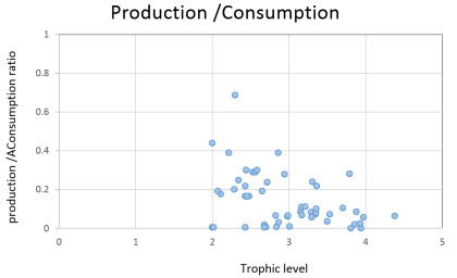
Production to Consumption ratio (P/Q) or the gross food conversion
| This indicates that a group cannot produce more than a fraction of what it has eaten, based on the 2nd law of thermodynamics (Link, 201). Because consumption is expected to be between three to ten times higher than production, in most cases, P/Q ratios will range between 0.05 to 0.3 (except for fast growing organisms and corals) as shown in the figure to the right. Most of the P/Q values of the 53 consumer groups in the model were within the range of 0.05 to 0.3 (except for turtle hatchlings, gastropods, squids, and salps). Groups with P/Q values higher than 0.3 were checked for data integrity before initiate the balance of the model. |
 |
Prior to final balance of the model, we checked that the model is in agreement with the basic thermodynamic rules of thumb described above. This diagnostic is only meant to be the first check of the model before begin the mass-balance process where further parameterization of some groups were conducted. A further diagnostics was run using the P/Q or the gross food conversion efficiency, indicating that the model follows the general ecological and thermodynamic rules. Once these underlying assumptions were tested with the PREBAL approach, we proceed to balance the model and re-checked again the PREBAL estimations to verify for incompatible vital rates of mortality (P/B) and consumptions (Q/B).
Ecotrophic Efficiency (EE)
We carried out a first run of the EwE model. We have used the EE values of the PREBAL EwE outputs as a preliminary diagnostic of the equilibrium assumption of the EwE model. EE is a measure of the proportion of production that is utilized by the next trophic level through direct predation or fishing. As a result, EE values should be between 0 and 1. Given a functional group, EE=0 indicates that the group is neither consumed by another group nor exported outside the model domain. Conversely, EE1 indicates that the group is heavily consumed (either preyed, grazed and/or fished), which allows no individuals to reach old age. The whole range of EE values can be found in Nature. However, values of EE>1 clearly indicate that the model dynamics is unrealistic. A number of unrealistic ecotrophic efficiencies were generated by the first run of the model in its PREBAL mode. Of these, approximately 40% of the groups out of balance (12 out of 29 groups) are represented by fish groups, indicating that we need more and better input data for these groups. As a result, in the next modelling stage, we focussed on mass-balancing first those groups with EE>1.
Model mass-balancing
The model was balanced using a series of iterative steps. During our first attempt to balance the Kimberley model, thirty-one of the 60 groups were thermodynamically. The model was balanced manually to ensure that changes to the input parameters were kept within biological reasonable limits. The first step was to reduce the predation on the groups that were out of balance, but maintaining the original values of biomass for groups with local biomass estimates by other WAMSI projects. The second step was to adjust consumption rates (Q/B) and production rates (P/B) to achieve mass-balance, where changes of less than 10% were applied to those groups out of balance. Finally, we minimized cannibalism within groups (i.e. large and small sharks, carnivore reef fishes) and liberate this energy to other groups (following Christensen et al. 2000). The basic input parameters of the mass-balanced Kimberley model are presented in Table 2.3.
It is important to mention that the process required to build the Kimberley EwE model is essentially open-ended. The parameters used in the model were revised and there is a possibility that new estimates along the project could replace some of the basic input parameters presented in Table 2.3.
Model calibration
The relative abundance (CPUE) and catch data required to calibrate the EwE Kimberley model were provided by the Department of Fisheries, Western Australia. The biomasses predicted by the model were fitted using time series data of relative abundance estimates of the main finfish species targeted in the Kimberley: Barramundi, Threadfin, Gold Snapper, Emperors, and Mackerel. This process known as tuning provides adjusted models that can track changes in abundance and CPUE that are known to have occurred in the past (see details in Christensen et al., 2005). In the Kimberley model, this required estimates of fishing mortality from 2010 to 2014 for these finfish species. The fishing mortalities for these species were calculated in the Ecopath base year as Fji0 = Yji0/Bi0, where Yji0 is the mean catch (2010-2014) of group i by fleet j, and Bi0 is the mean biomass during the year (estimated by depletion techniques). The differential equations that express flux rates among biomass pools as a function of time varying biomass are solved by an Adams-Bashford method of integration (this method is a faster and more stable integration routine than the Range-Kutta 4th Order, see details in Christensen et al., 2005). The predicted CPUE (as relative abundance) of the main five finfish species target in the Kimberley resulted of the calibration of the Kimberley model is shown below
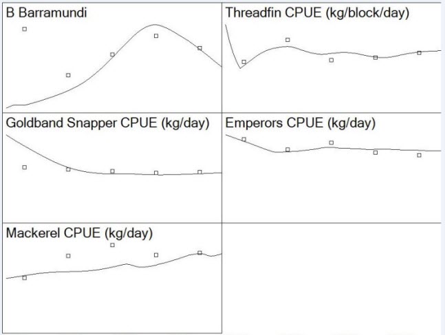 |
| Figure 5. Calibration of the EwE Kimberley model displaying the predicted biomass and CPUE of the main five finfish species target in the region (line) and the biomass and CPUE reported by Department of Fisheries, Western Australia |
Ecospace: Dynamic Spatial Modelling
The dynamic food web simulations of Ecosim run in parallel in linked square map grid cells. Biomass in each functional group in the model transfers between cells according to a set of dispersal rules, with relative movement speeds depending on food availability and predation risk (Christensen and Walters, 2004). Fisheries in the model occur in regions where catch rates for the target species are maximised and can be excluded from defined regions of cells, emulating spatial management of marine parks. Exclusion of all of the fisheries in the model represents a no-take MPA (sanctuary area).
This section reports dynamic simulations of the Kimberley food web (Ecopath with Ecosim, EwE) model used to create a spatial model with habitats, fisheries and management areas (marine parks including sanctuary areas).
Habitats
| The Kimberley Ecospace model comprises an area of approximately 93,000 km2. This ecosystem is represented by a grid of 3,600 cells (60 x 60 cells) of 25 km2 each. The Ecospace habitat base map (Figure A) was designed based on the detailed marine biological survey carried Edmunds and Mustoe, 2001; by Fry et al. 2008, Llewellyn and Gamblin, 2008; Watson et al., 2009 (Montara oil spill); Heyward et al 2010 & 2011; Montara Environmental Monitoring Program 2013; Comrie-Greig and Abdo, 2014. Using this comprehensive survey, it was possible to include the fourteen major habitat types within the region. 15 Habitats were defined based on Fry 2008; Woodside Reports; INPEX Reports and WAMSI (Figure 1) |
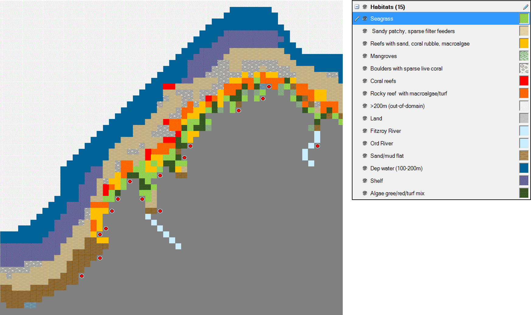 Figure 1. Main habitats defined in the Ecospace model (click to view larger image) Figure 1. Main habitats defined in the Ecospace model (click to view larger image) |
- Seagrass (SA)
- Sandy patchy, sparse filter feeders (SP)
- Reefs with sand, coral rubble, macroalgae (R )
- Mangroves (M)
- Boulders with sparse live coral (B)
- Coral reefs (C )
- Rocky reef with macroalgae/turf (RM)
- >200m (D)
- Fitzroy River (FR)
- Ord River (OR)
- Sand/mud flat (S)
- Deep water (100-200m; DW)
- Shelf (S)
- Algae green/red/turf algae mix (A)
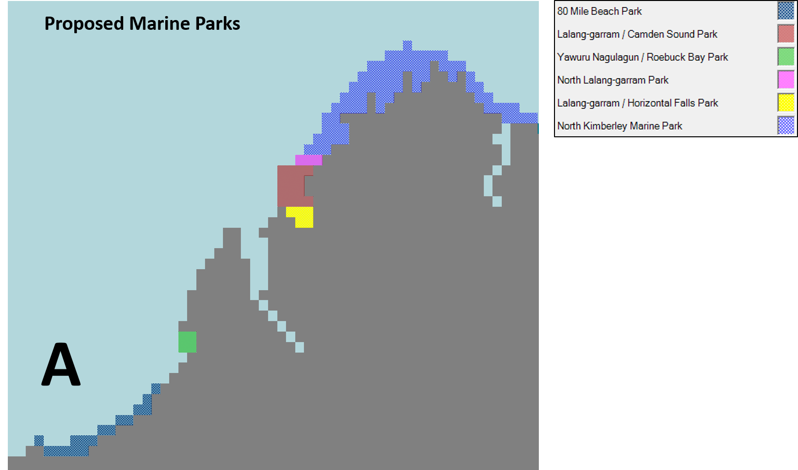
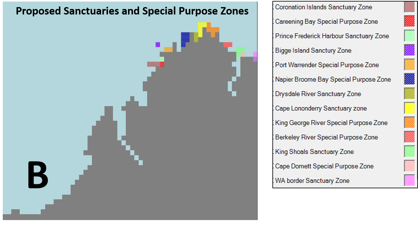
Zoning: Marine Parks & Special Purpose Areas
In addition to the fourteen habitat types considered in the model, three types of protected areas were included in the zoning map. These zones or protected areas were defined:
- Six proposed Marine Parks: 80 Mile Beach Park, Lalang-Garram/CamdenSound Park, Yawuru Nagulagun/Roebuck Bay Park, North Lalang-garram, Lalang-garram Park, Lalang-garram/Horizontal Fallas park, and North Kimberley Park.
- Seven proposed Sanctuary Zones (no commercial/recreational fishing allowed): Coronation Island, Prince Frederick Harbour, Bigge Island, Drysdale River, Cape Lononderry, King Shoals, and Western Australian border.
- Six proposed Special Purpose Zones (recreational fisheries allowed): Careening Bay, Port Warrender, Napier-Broome Bay, King George River, Berkeley River, and Cape Dommett.
The Sanctuary Zones and Special Purpose Zones (Scientific Reference) included in the model are presented in Figure 2.
Human use of the Kimberley coast
Ecospace diagnostics: Habitat capacity
in the form of a GIS-like layer for each species group, Ecospace determines its relative abundance (biomass) in the food web operating in each spatial cell at the end of the 35-year run (2050). Movements between cells was based on species dispersal rates and quality of adjacent habitats.
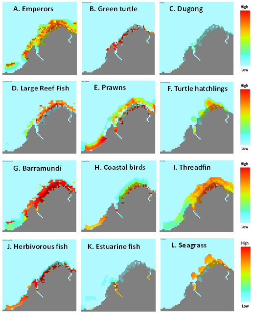 |
| Figure 4. Twelve examples of Ecospace habitat capacity maps (red is the highest relative habitat suitability; blue is no suitability): A. Emperors; B. Green turtle; C. Dugong; D. Large Reef Fish; E. Prawns; F. Turtle hatchlings; G. Barramundi; H. Coastal birds; I. Threadfin; J. Herbivorous fish; k. Estuarine fish; and L. Seagrass (click to view larger image) |
Ecospace Diagnostics: potential fishery intensity
There are currently no established routines for testing, calibrating and validating Ecospace outputs against spatial reference data or time series of forcing functions to drive the simulations. However, the spatial distribution of target species (probably the best known species in the region) were used as a diagnostic tool to evaluate its performance. These maps (Fig. 5) are based on fishing effort distribution obtained from: 1) DoF catch maps reported for commercial fleets (2010-2016); and by 2) Recreational fishing effort provided by DoFWA 2017. When the dynamic Ecospace model runs, fishery catches are determined by the fishing gear (target species, bycatch and pollution-target species) and relative biomass abundance of these target species moderated by the relevant potential fishing intensity maps.
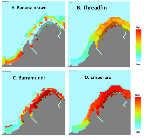 |
| Figure 5. Four examples of Ecospace potential fishery intensity maps (red is the highest relative potential fishing intensity; blue is no fishing): A. Banana prawn; B. Threadfin; C. Barramundi; and D. Emperors. (click to view larger image) |
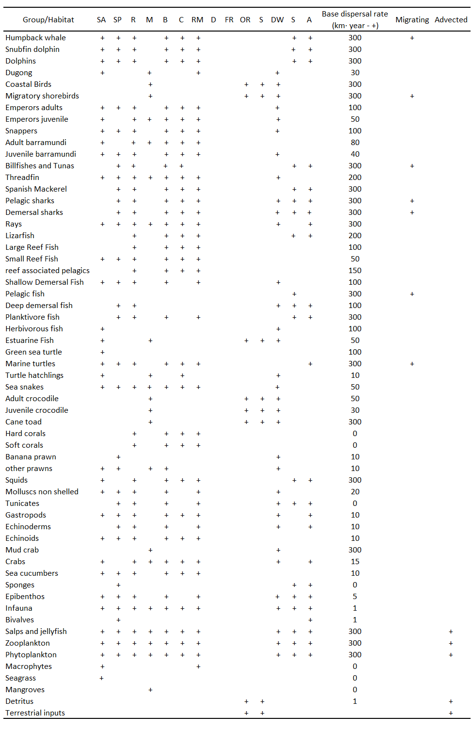
Base dispersal rate, migration and advection
Due to the lack of specific information on dispersal, the base dispersal rates have been set according to the general scheme used by Loneragan et al 2011 and Lozano-Montes et al (2011). Therein, the dispersal rates of functional groups are set according to their general type: marine mammals, 300 km·yr-1; sea birds, 300 km·yr-1; pelagic fish, 300 km·yr-1; demersal fish, 30 km·yr-1; benthic invertebrates, 3 km·yr-1; plankton, 300 km·yr-1; detritus, 3 km·yr-1; turtles, 300 km·yr-1; and pelagic invertebrates, 300 km·yr-1 (Table 1). The advection field for the Kimberley Ecospace model has been set according to Ming et al.(2017) flow field distribution of average depth in 2015. Salps, Jellyfish, zooplankton, phytoplankton, detritus and terrestrial inputs are set as advected groups.
 |
| Figure 5. Four examples of Ecospace potential fishery intensity maps (red is the highest relative potential fishing intensity; blue is no fishing): A. Banana prawn; B. Threadfin; C. Barramundi; and D. Emperors. (click to view larger image) |
References
- Beckley, L.E. 2015. Human use patterns and impacts for coastal waters of the Kimberley. Western Australian Marine Science Institution, Perth, Australia. Final Report. 98p.
- Christensen, V., and Walters, C. 2004. Ecopath with Ecosim: methods, capabilities and limitations. Ecological Modelling 172(2–4): 109–139.
- Christensen, V., Walters C.J. and Pauly, D. 2005. Ecopath with Ecosim: a User’s guide. Fisheries Centre of
University of British Columbia, Vancouver, Canada. 154 pp.
- Comrie-Greig, J. and Abdo, L (eds). Ecological studies of the Bonaparte Archipelago and Browse Basin. INPEX Operations Australia Pty Ltd, Perth, Western Australia. 132p
- Edmunds, M., and Mustoe, S. 2001. Coastal and Marine Natural Values of the Kimberley. Produced for WWF-Australia by: AES Applied Ecology Solutions. Melbourne, Victoria. Australia. 259p.
- Fry, G., Heyward, A., Wassenber, T., Taranto, T., Keesing, J., Irvine, T., Stieglitz, T., Colquhoun, J. 2008. Benthic habitat surveys of potential LNG hub locations in the Kimberley region. A study commissioned by the Western Australia Marine Science Institution on behalf of the Northern Development Taskforce. Final Report. CSIRO-AIMS. 89p
- Heyward, A. Tinker, P., Btooks, K., Suosaari, G., Johns, K., Oliver, J. 2010. Monitoring programs for the montara Well release Timor Sea: Final Report on the Nature of Barracouta and Vulvan Shoals. Final Report for PTTEP Australasia Pty/Ltd. 49p.
- Heyward, A., Jones, R., Meeuwig, J., Burns, K., Radford, B., Fisher, R., Meekan, M., Stowar, M., 2011. Montara: 2011 offshore Banks assessment survey. Final report by the Australian Institute of Marine Science for PTTEP Australasia (Ashmore Cartier) Pty.Ltd. 000/2011/02-04.
- Llewellyn, G. and Gamblien, P. 2008. Coastal and Marine Natural values of the Kimberley. Report for WWF-Australia. 60p.
- Ming, F., Slawinski, D., Shimizu, K., Zhang, M. 2017. Climate change: knowledge integration and future projection. Western Australian Marine Science Institution, Perth, Australia. Final Report. 79p.
- Montara Enviromental Monitoring Program. 2013.A new body of world class research on the Timor Sea. Research Report. PTTEP Australiasia. 112p.
- Watson, J.E.M., Joseph, L.N. and Watson, A.W.T. 2009. A rapid assessment of the impacts of the Montara field oil leak on birds, cetaceans and marine reptiles. Prepared on behalf of the Department of the Environment, Water, Heritage and the Arts by the Spatial Ecology Laboratory, University of Queensland, Brisbane.
|