The BathLab - Quick Guide

1. Installation
2. Purpose

1. Define the strength of the Inflow and Outflow
2. Run the BathTub dynamics for a certain amount of time steps
3. Observe the level of Stock in the container
4. Optionally, you can save and load settings for specific training exercises

Purpose

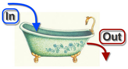
This interactive model is designed to train on a simple dynamical system involving stocks & flows. While the specific aim of the training will be set by the facilitator, in general you will be asked to predict the amount of material in the central image (a container holding the stock of a certain material) as a function of how much material enters the container (from the top left box) and exits the container (from the bottom right box). At any given time, the amount in the container (Stock) is equal to the stock at the previous time step, plus the Inflow, minus the Outflow, that is:

Stock(next time step) = Stock(now) + Inflow(now) - Outflow(now)

As explained in Sweeney & Sterman (2000), even well educated people often fail at predicting the behaviour of this apparently simple process.

In the rest of the document we call BathLab the interactive model and BathTub dynamics the evolution of the above equation.

Sweeney, L. B., & Sterman, J. D. (2000). Bathtub dynamics: initial results of a systems thinking inventory. System Dynamics Review, 16(4), 249-286.

Define the strength of the Inflow and Outflow

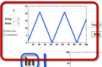
The flows are visualised and controlled via the panels at the top-left (Inflow) and bottom-right (Outflow). The Inflow panel is shown in Figure (2a); the Outflow panel works in exactly the same manner.

Each panel is divided into two sub-panels:

1. The visualisation panel (Figure 2b)
2. The control panel (Figure 2c)

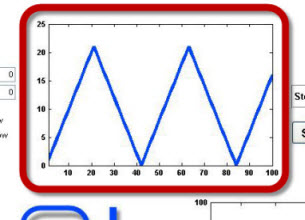
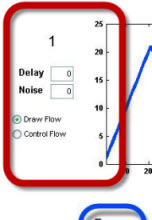
Figure 2a		Figure 2b		Figure 2c

The visualisation panel displays on the X axis the time throughout the dynamics (from time step 1 to time step 100) and on the Y axis the intensity (or strength) of the Flow.

When you load the BathLab you will see a time series plotted on this panel (blue for Inflow and red for Outflow as in Figure 2a). These represent how the flows will vary in time.

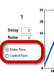
The Control Panel allows you to change/control the flow in two different modes: ‘Draw Flow’ and ‘Control Flow’. In the default setting, you will see the option “Draw Flow” ticked (Figure 3a). This setting allows you to change the flow plot by drawing your own time evolution. To do so:

1. point the cursor over the plot
2. Left-click to input a few points; the chosen points will be shown in the panel
3. Shift+Left-click to complete the flow time series. This will draw a line as a cubic-spline interpolation of the chosen points.

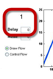
During the model run, the number above the ‘Delay’ field shows the current value of the flow strength (Figure 3b).

In this setting you can also:

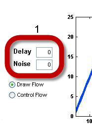
• add Noise to the flow strength by typing on the Noise field (Figure 3c). This value represents the maximum amplitude of an additive white noise, which is added to the flow at each time step.
• impose a Delay to the flow time evolution by typing on the Delay field (Figure 3c). This value represents how many time steps need to occur before any change in the flow impacts the Stock in the container.

Figure 3a		Figure cb		Figure 3c

If you tick “Control Flow” (see Figure 3a) you can control the flow in a step by step mode. After clicking “Control Flow” you will see that a) the ‘Draw Flow’ button disappears and b) a slider appears. Now you can

• Change the flow strength at the current time step using the slider (the change will appear in the field in Figure 3b)
• Change the flow strength by directly typing on the field in Figure 3b.

The new value of the flow strength will then be used in the model run until the value is changed again. Notice that to go back to the “Draw Flow” mode, the simulation needs to be re-initialised by clicking on “Clear” (see below).

Run the BathTub dynamics for a certain amount of time steps

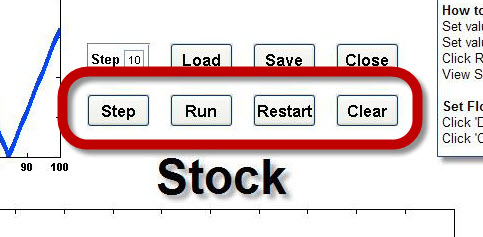
The BathLab run can be controlled via the buttons immediately above the central plotting area, as highlighted in Figure 4.

• Step carries out the simulation for one time step and pauses for user input;
• Run completes the simulation from the current time to the final step; then awaits user input
• Restart clears the time series plot and allows you to restart the simulation from the start. It does not reset the In and Out flows and does not clear your drawing on the time series plot
• Clear clears all time series plots, and all parameter changes. It is equivalent to closing the program and re-launching it.

Figure 4

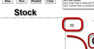
Observe the level of Stock in the container

As for the flow visualisation plots, the Stock panel displays on the X axis the time thought the dynamics (from 1 to 100 time steps) and on the Y axis the level of the Stock (how much material is in the container). The Stock level at the current time is also displayed at the top-right of the plot (see Figure 5). The Stock value cannot be changed or edited in the panel, since it is determined solely by the strength of the Inflow and Outflow. In order to help the interaction between the facilitator and the user(s) and to test the learning you can draw lines over the Stock plot. This allows, for example, to draw the expected or desired behaviour of the Stock, which can then be compared to the actual output of the run. To draw the line:
		Figure 5

1. point the cursor over the time-series plot
2. Left-click to input a few points; the chosen points will be shown in the panel
3. Shift+Left-click to complete the line. This will draw the line as a cubic-spline interpolation of the chosen point
4. Right-click on the line allows to change the line colour or to delete the line. Notice that this is the only way to delete the line, since it will not be deleted when the button Clear is pressed)
5. More lines can be drawn with the same procedure

Back to Manual table of contents

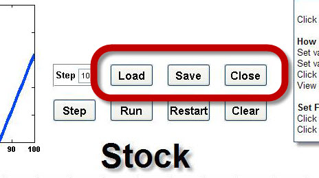
Save and load user-defined settings

You can load and save the settings via the buttons shown in Figure 7. The settings are saved as a structure in a Matlab file (.mat) and include: The availabe buttons provide for the following: Load: loads a pre-saved setting file and resets all parameters Save: saves the current parameters Close: quits APE and closes the GUI. Back to Manual table of contents
		Figure 6

Download BathLab Model

Notice, currently the model runs only on PC.

To use this model you first need to install the MATLAB Compiler Runtime (MCR) on you PC (see information on the MCR):

• download MCRInstaller.exe (150Mb, be patient)
• run it - this will install the MCR
• the entire operation will take a few minutes, but you need to so it only once.

Once you have installed your MATLAB Compiler Runtime (MCR):

• download the BathLab model
• unzip the folder
• run BathLab.exe
• the first time you run the model, it will extract some files; this may take a few seconds but this also will be done only once.