Activity People Environment

A simplified and general model to study the dynamics of the interaction between
people, their activities and the environment

Introduction Documents Download Draft Technical Manual Interactive APE Manual   Fabio Boschetti & Nicky Grigg

Introduction - The Model

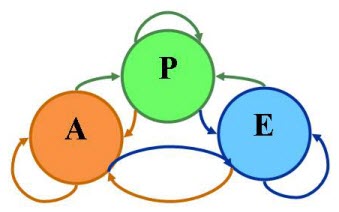
A number of resource exploitation problems can be reduced to the interaction between three abstract variables: the size of the exploiting population, the way exploitation is carried out and the dynamics of the environment which provides the resource. We have developed a simplified and general model (APE, for Activity, Population and Environment) to study the dynamics of such interactions. By specifying the nature of the A, P and E state variables, this abstract representation can be applied to a range of different problems, for example:

• climate change (A=wealth generation, P=population dynamics, E=cumulative CO2);
• water management (A=agriculture, P=population dynamics, E=water availability and quality);
• tourism development (A=tourism infrastructure development, P=number of tourists, E=environment quality and attractiveness);
• fishery management (A=type of fishing activity, P=fishing fleet size, E=fishing stock health).

Seen as simple three-node networks, the global dynamics of the different APE models differ depending on the local dynamics of the three state variables (for example on whether E is renewable or not), on the functional form and strength of the links and, crucially, on their signs which determine the presence of positive or negative feedback loops.

Motivation

While a simple APE model can not capture the complexity of a real system, it can represent how people think of, discuss and take decisions about it: studies in cognitive science report that humans (experts included) are rarely capable of reasoning about more than a few variables interacting over more than 2-3 cycles. To circumvent this cognitive limitation, an APE model helps us study the medium and long-term behaviour of simple systems. This allows interested parties to develop an intuition for the role and impact of specific links on system behaviour and for where points of intervention may lie. An APE model can thus be seen as a learning tool, a communication and collaboration tool, and a reality check to verify the soundness of assumptions about system behaviour.

Model modes

The APE model can be run in two modes: • in the interactive mode simple menus allow users to modify the nature of the links and of the internal dynamics of the state variables and to observe the resulting global system dynamics. This can be carried out by individual users, thereby providing ‘hands-on’ learning, or by teams fostering communication and decision making in a 'companion model' setting; • in the non-interactive mode, numerical optimisation routines and ensemble runs can be used to detect the different dynamical behaviours a specific APE model can exhibit thus, for example, informing policy-makers on the range of scenarios a policy may need to address.

Back

Documents

Back

Download APE Model

Notice, currently the model runs only on PC.

To use this model you first need to install the MATLAB Compiler Runtime (MCR) on you PC (see information on the MCR):

• download MCRInstaller.exe (150Mb, be patient)
• run it - this will install the MCR
• the entire operation will take a few minutes, but you need to so it only once.

Once you have installed your MATLAB Compiler Runtime (MCR):

• download the APE model
• unzip the folder
• run InteractiveAPE.exe
• the first time you run the model, it will extract some files; this may take a few seconds but this also will be done only once.

Back

Interactive APE

1. run a simulation with the APE model
2. define the APE model parameters (impacts and internal dynamics)
3. define the simulation parameters (simulation start time, end time, step interval and added noise)
4. define the initial conditions for the simulation
5. save and load user-defined settings
6. draw lines over the time-series plot.

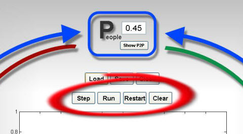
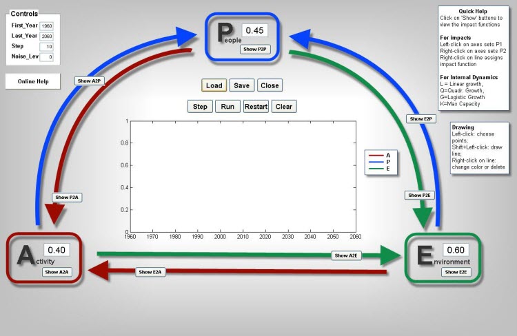
Run a simulation with the APE model

To install the program in your computer, follow these steps. To launch the GUI, double click on the program 'InteractiveApe.exe'. Your APE run can be controlled via the buttons immediately above the central plotting area, as highlighted in Figure 2.

Figure 2

• Step carries out the simulation for one time step and pauses for user input;
• Run completes the simulation from the current time to the Final Year; then awaits user input
• Restart clears the time series plot and allows you to restart the simulation from the First Year. It does not reset the model parameters and does not clear your drawing on the time series plot
• Clear clears the time series plot, your drawings and all parameter changes. It is equivalent to closing the program and re-launching it.

Define the APE model parameters

Figure 3a		Figure 3b

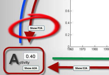
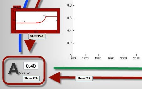
You can change the way the state variables (A, P and E) affect one another. As an example, we focus on how P affects A. Click on the Show P2A button, as in Figure 3a. A new Panel will appear as in Figure 3b. This panel shows the impact function of P on A. By pointing the mouse on the panel you can modify this function as follows:

• Left-Click resets point P1
• Right-Click resets point P2
• Right-Click over the line allows you to choose the transition between P1 and P2.

Clicking again on the Show P2A button closes the panel in Figure 3a.

Figure 4a		Figure 4b

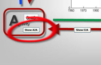
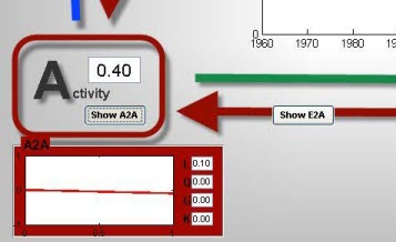
Similarly, you can change the way the state variables’ internal dynamics, that is they way they would evolve if undisturbed. As an example, we focus on A. Click on the Show A2A button, as in Figure 4a. A new panel will appear as in Figure 4b. This panel shows A’s internal dynamics function. To modify assign values to these parameters:

• L= linear growth coefficient
• Q= quadratic growth coefficient
• G= logistic growth coefficient
• K= maximum capacity in logistic growth.

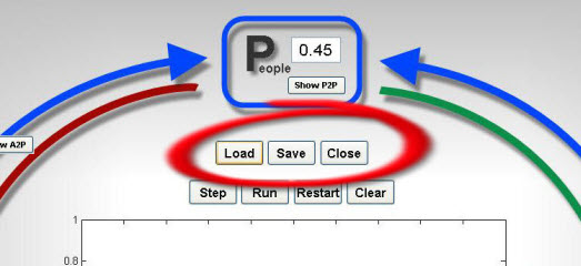
By assigning a zero values to certain parameters you can choose between linear, quadratic or logistic growth, as well as any combination. Clicking again on the Show A2A button closes the panel in Figure 4a.

Back to Manual table of contents

Save and load user-defined settings

You can load and save APE setting via the buttons below the P panel as in Figure 5. The APE settings are saved as a structure in a Matlab file (.mat) and include:

• the impact functions and their parameters
• the internal dynamics functions and their parameters
• the simulation parameters (simulation start time, end time, step interval and added noise) and
• the initial conditions.

Figure 5

The availabe buttons provide for the following:

• Load: loads a pre-saved setting file and resets all parameters
• Save: saves the current parameters
• Close: quits APE and closes the GUI.

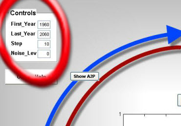
Back to Manual table of contents

Define the simulation parameters

You can change the parameters controlling the simulation via the panel named Control on the top left, as in Figure 6. In particular:

• First Year sets the simulation starting time
• Last Year sets the simulation end time
• Step sets the time step for running the simulation step by step
• Noise Lev sets the optional noise level to add to the simulation. It represents the maximum amplitude of a additive white noise, which is added to the rate of change of A, P and E.

Figure 6

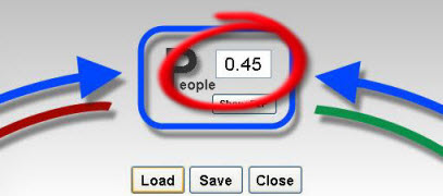
Back to Manual table of contents

Define the initial conditions

The value of the A, P and E state variable can be changed at any time before and during the simulation by typing of the area as shown in Figure 7. Doing this before the start of the simulation allows to set the initial conditions. Doing so during the simulations allows to model instantaneous forcing to the system.

Figure 7

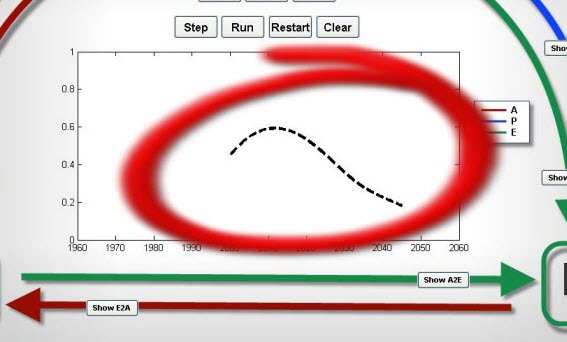
Back to Manual table of contents

Draw lines over the time-series plot

You can draw lines over the time-series plot. This allows, for example, to draw the expected or desired behaviour of one or more state variables, which can then be compared to the actual output of the simulation. The line will be drawn dashed as in Figure 8. To draw the line:

1. point the cursor over the time-series plot (see Figure 8)
2. Left-click to input a few points; the chosen points will be shown in the panel
3. Shift+Left-click to complete the line. This will draw the line as a spline interpolation of the chosen point (oscillations should be expected if close points with large gradients are chosen)
4. Right-click on the line allows to choose a line color (red, blue or green, as used to plot the A, P and E time series) or to delete the line (the line will also be deleted when the button Clear is pressed)
5. More lines can be drawn with the same procedure

Figure 8

Back to Manual table of contents